
TEMPLATES & BUSINESS WORKFLOWS
How to Create a Dependent Drop-Down List in Excel
Choose a department, then show only its matching items in the next Excel drop-down. This beginner-friendly setup uses a source table, two short formulas, and named ranges—no VBA required.

The idea in one minute
A dependent drop-down is a pair of lists: the first cell chooses a group, and the second list changes to match. We’ll use Department in OrderForm!B2 and Item in OrderForm!C2. A helper formula filters the choices in the background; a workbook name lets Data Validation use that changing list.
If you’ve used a drop-down to control a chart, the same “selection drives the result” idea is at work here. See how a drop-down can drive a dynamic Excel chart.
1. Put each choice on its own row
On a sheet named Lists, create two columns named Department and Item. Use one row for every valid pair:
| Department | Item |
|---|---|
| Finance | Monthly Report |
| Finance | Budget Template |
| Finance | Invoice Log |
| HR | Leave Calendar |
| HR | Onboarding Checklist |
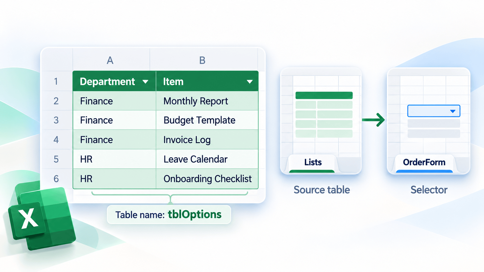
tblOptions so new rows are easier to include.- Select a cell in the list and press Ctrl + T on Windows or ⌘ + T on Mac.
- Confirm My table has headers, then choose OK.
- On Table Design, change the table name to
tblOptions.
Department and Item, and its name is tblOptions.2. Build the Department drop-down
On Lists, enter this in cell D2. It creates a sorted list with each department shown once:
=SORT(UNIQUE(tblOptions[Department]))Next, give the spilled results a workbook name:
- Choose Formulas → Name Manager → New.
- Name it
DepartmentChoices. In Refers to, enter=Lists!$D$2#, then save. - Select
OrderForm!B2and choose Data → Data Validation. - Set Allow to List, set Source to
=DepartmentChoices, and choose OK.
Click B2. You should be able to choose Finance or HR. The # after D2 means “use the full spilled list,” even if it grows.
3. Filter the Item choices
On Lists, enter this formula in F2. It reads the selection in B2, returns only matching items, removes duplicates, and sorts the result:
=IF(OrderForm!$B$2="","",SORT(UNIQUE(FILTER(tblOptions[Item],tblOptions[Department]=OrderForm!$B$2,""))))When B2 is Finance, F2 spills Budget Template, Invoice Log, and Monthly Report. Choosing HR changes the spill to its two items.
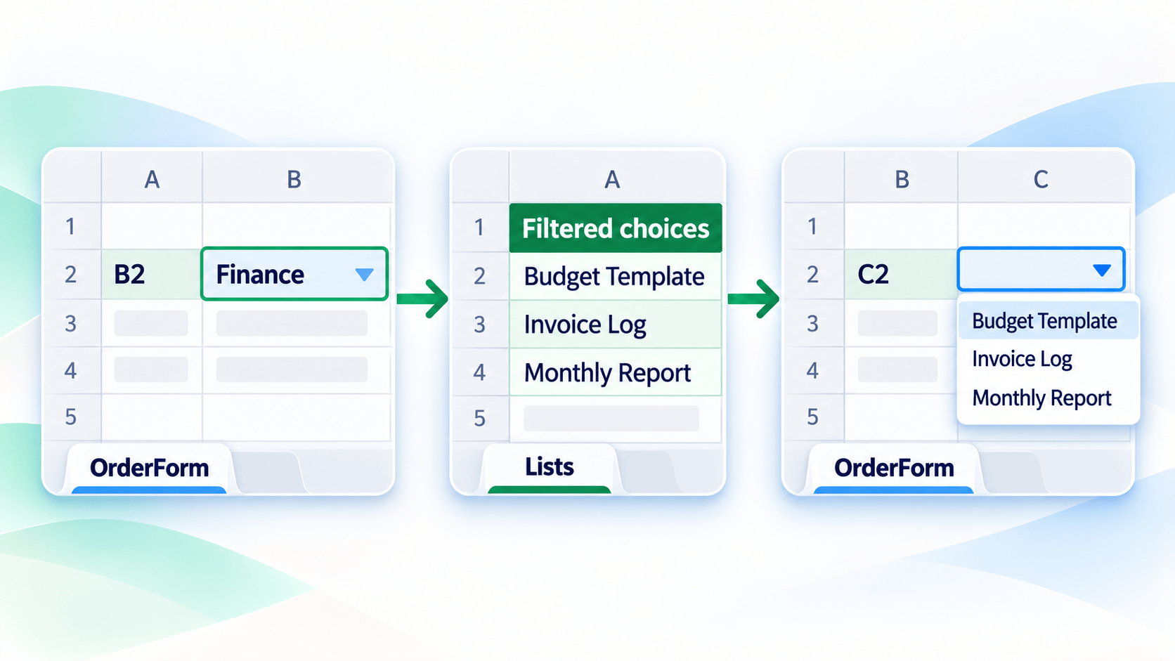
To connect the filtered list to the second drop-down, create another workbook name: go to Formulas → Name Manager → New, name it ItemChoices, and set Refers to to =Lists!$F$2#.
Select OrderForm!C2, open Data → Data Validation, set Allow to List, and set Source to =ItemChoices. Choose OK. Now C2 should offer the items for the department selected in B2. Using a workbook name also avoids entering a direct cross-sheet spill reference in the validation box.
4. Test it before using the form
- Choose Finance in B2 and confirm C2 has three Finance items.
- Change B2 to HR and confirm the choices in C2 update.
- Add a new Finance row to
tblOptions; check that it appears in the helper list and C2. - After changing B2, clear any old value in C2 before choosing again. Data Validation changes the next choices; it does not erase a value already entered.
| If you see… | Check this |
|---|---|
#SPILL! in F2 |
Clear the cells below F2 and make sure the formula is outside the Table. |
| The helper list is blank | Check that B2 matches a Department value exactly, including spaces. |
| An old item remains in C2 | Clear C2 after changing the department, then choose a new item. |
If your Excel version doesn’t have FILTER and UNIQUE
For older Excel versions, create a named range for each department’s items, such as Finance and HR. Set C2’s Data Validation Source to this formula:
=INDIRECT(SUBSTITUTE($B$2," ","_"))The names must match the department labels; replace spaces in a label with underscores in its range name. This fallback is handy for a small, stable list. The Table and FILTER method is easier to extend.
For related skills, see how to return a live list with FILTER and how UNIQUE removes repeated values. Microsoft’s drop-down list guide covers the Data Validation settings, and its spilled-range operator guide explains the # reference.
Frequently asked questions
Can I do this without VBA?
Yes. The modern method uses formulas, workbook names, and Data Validation. It doesn’t need VBA in Excel versions that support FILTER, UNIQUE, and SORT.
Why doesn’t the second list clear when I change the first?
Data Validation controls what you can enter next; it doesn’t remove an existing cell value. Clear C2 after changing B2.
Build cleaner Excel forms
Browse the OneXcel Tutorial Hub for practical formulas, templates, and workflow guides.