How to Filter a Dynamic List with the FILTER Function

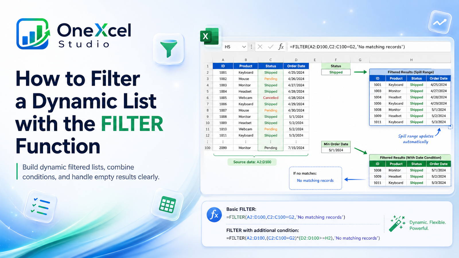
The FILTER function creates a new list containing only the rows that meet your condition. In current Excel versions, the result can spill into the cells below and beside the formula automatically, so you do not copy the formula down row by row. Start with one clear condition, confirm the returned rows, then add more criteria only when needed.

Build the FILTER dynamic-array function formula

Assume a source table is in A2:D100, Status is column C, and the selected status is in G2.

=FILTER(A2:D100,C2:C100=G2,"No matching records")

A second useful version is:

=FILTER(A2:D100,(C2:C100=G2)*(D2:D100>=H2),"No matching records")

FILTER returns every row where the include test is TRUE. Multiplication combines conditions as AND; addition can be used for OR when the logical tests are converted to ones and zeros.

Step-by-step formula workflow

1. Choose a clear source range with matching row counts.
2. Create one logical test and confirm it returns TRUE and FALSE correctly.
3. Use that test as the FILTER include argument.
4. Add a useful if-empty message.
5. Leave enough blank space for the results to spill and test changes to the source.

Common formula mistakes

Mistake	Why it matters
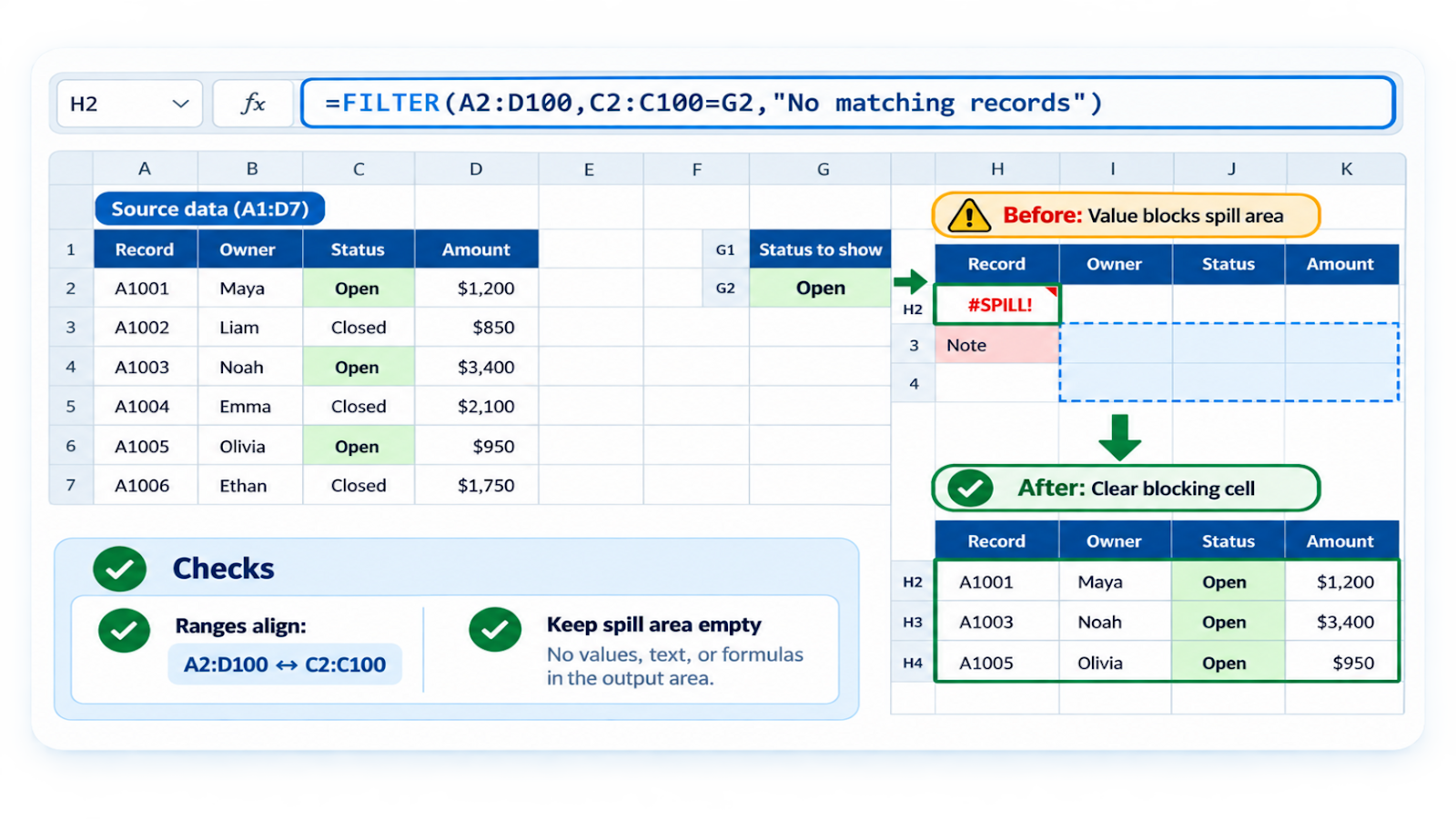
Blocking the spill range	Any value inside the output area causes #SPILL!.
Using include ranges of different heights	The logical tests must align with the returned rows.
Returning entire columns unnecessarily	Large spill formulas can slow the workbook.
Ignoring blanks in the source	Blank rows may appear when the source range is larger than the data.
Assuming FILTER exists in old versions	It requires a version that supports dynamic arrays.

Worked FILTER example with AND and OR

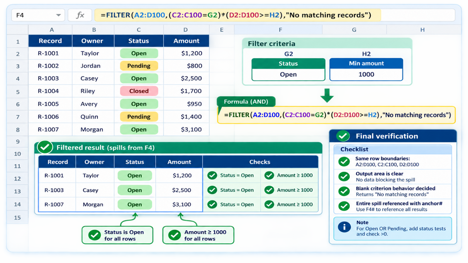
Suppose G2 contains Open and H2 contains 1000. The formula =FILTER(A2:D100,(C2:C100=G2)*(D2:D100>=H2),"No matching records") returns only rows that are both Open and at least 1000. If the rule should return Open or Pending rows, combine the status tests with addition and test that the result is greater than zero.

When the source is an Excel Table, structured references make the formula easier to maintain as rows are added. Keep the output area clear and avoid typing directly inside the spill result. If another formula needs the entire result, reference the spill anchor with #. Also decide how blanks should behave before combining conditions; an empty criterion cell can unintentionally filter out every row unless the formula explicitly treats blank as “all.”

Frequently asked questions

How do I combine two conditions?

Multiply the Boolean tests for AND or add them for OR, then test the result.

Can FILTER return selected columns only?

Yes. Point the array argument to the columns you want or combine it with CHOOSECOLS in supported versions.

Why do I see #CALC!?

No records matched and the optional if-empty argument was omitted.

Will it update automatically?

Yes. The spilled result recalculates when the source data or criteria change.