
Shortcuts & Faster Workflows
How to Freeze Panes Like A Pro
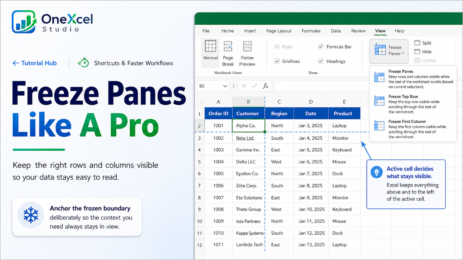
Freeze Panes is most useful when it preserves the context needed to interpret a record. The trick is not simply turning the command on; it is selecting the correct anchor cell so the header row, identifier column, or both remain visible while you scroll.
Start with the right worksheet setup
Open a sheet with a header row and several identifying columns. Decide what must stay visible: the top row, the first column, or a block such as rows 1:2 and columns A:B. Excel freezes everything above and to the left of the active cell, so the cell position is the key decision.
Work through the Excel example
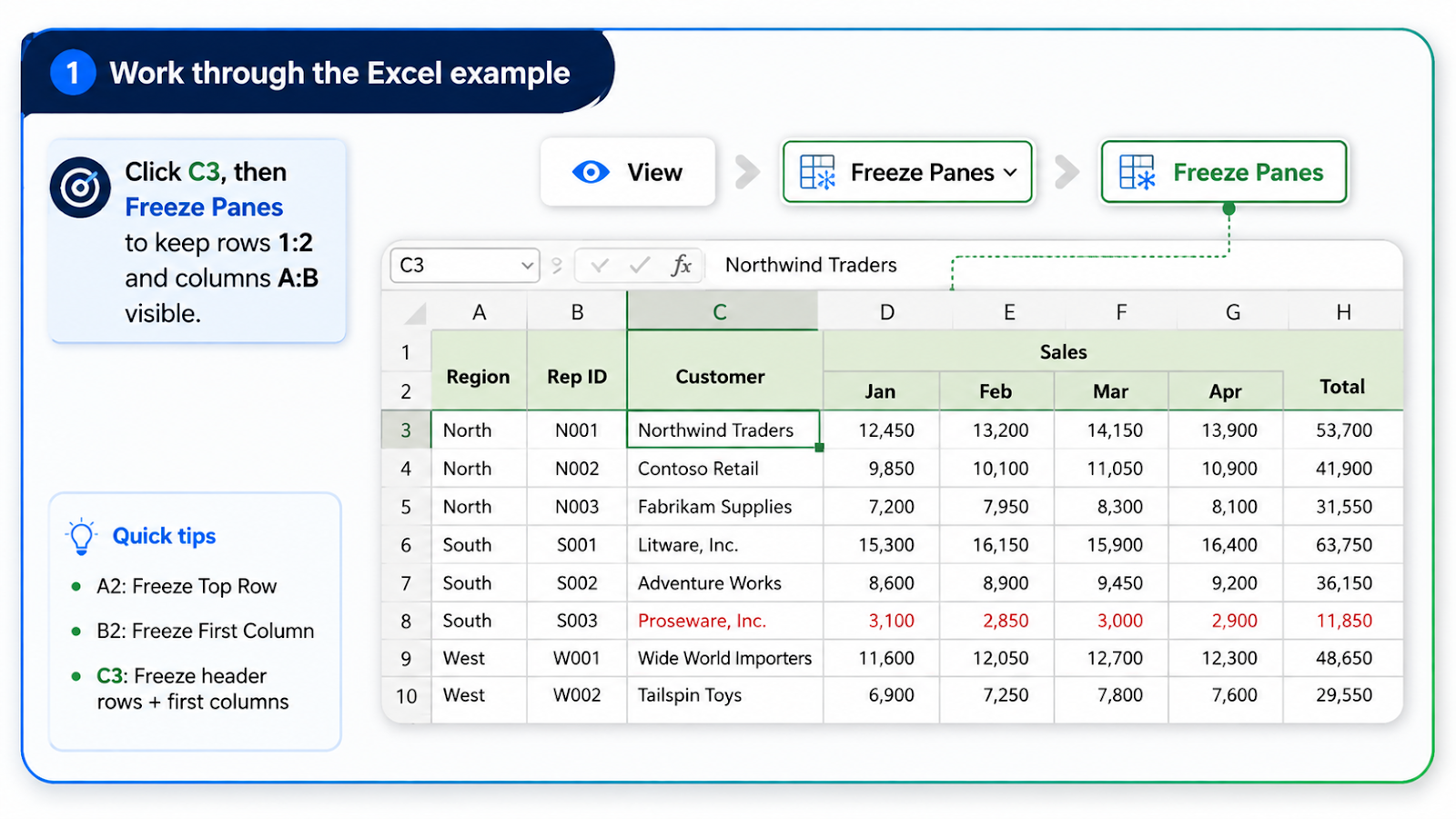
To keep only the header row, click A2 and choose View > Freeze Panes > Freeze Top Row. To keep the first column, use View > Freeze First Column. To keep both the header and the first identifier column, click B2 and choose View > Freeze Panes > Freeze Panes. For a two-row header and two identifier columns, click C3 before selecting the same command. Excel will keep rows 1:2 and columns A:B visible.
Keep the original values visible, test a normal case and an exception, then compare the output with the business rule the worksheet is meant to represent.
Verify the result and protect the workflow
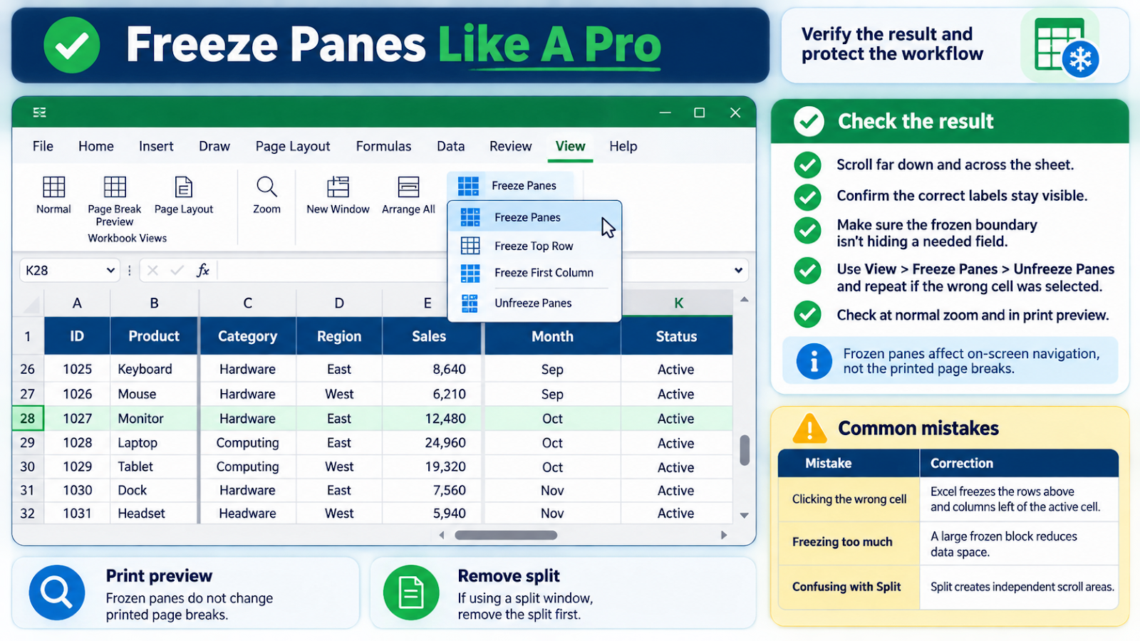
Scroll far down and across the sheet. For large tables, the Ctrl + Arrow navigation guide can help you move through contiguous data efficiently. Confirm that the correct labels remain visible and that the frozen boundary is not hiding a needed field. Use View > Freeze Panes > Unfreeze Panes, then repeat the setup if the wrong cell was selected. Check the sheet at normal zoom and in print preview; frozen panes affect on-screen navigation, not the printed page breaks. If the worksheet uses a split window, remove the split before judging the result. When filters are part of the workflow, review the Ctrl + Shift + L filtering guide as a related check.
Common mistakes and corrections
| Mistake | Correction |
|---|---|
| Clicking the wrong cell | Excel freezes the rows above and columns left of the active cell, so the anchor must be deliberate. |
| Freezing too much | A large frozen block reduces the space available for the actual data. |
| Confusing Freeze Panes with Split | Split creates independent scroll areas; Freeze Panes keeps a fixed context. |
| Forgetting the final view | Leave the sheet positioned where a reader can understand the first visible records. |
Frequently asked questions
Can I freeze both rows and columns?
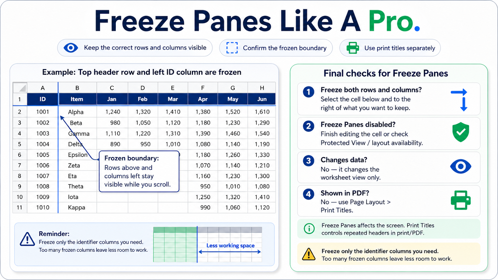
Yes. Select the cell immediately below and to the right of the areas to preserve.
Why is Freeze Panes disabled?
You may be editing a cell, using a protected view, or working in a layout where the command is unavailable.
Does it change the data?
No. It changes the worksheet view only.
Do frozen panes appear in PDF output?
No. Use print titles or page setup when repeated print headers are needed.
For related practical lessons, continue through the OneXcel Tutorial Hub and the free Excel resources.
Use panes with print and edit decisions
Freeze Panes affects the screen, not the printed report. If the same header must repeat on every printed page, use Page Layout > Print Titles and set the rows to repeat at the top. This is a separate setting, so a worksheet can have a frozen header for editing and a repeated header for PDF output.
For a wide data table, freeze only the identifier columns that help the user understand a row. Freezing five or six columns may technically preserve context but leave too little room for the current data. If the worksheet has a title block above the table, count those rows carefully before choosing the anchor cell.
When reviewing someone else’s workbook, unfreeze and reapply the panes in a copy rather than guessing from the visible boundary. A frozen view can hide a column or row that the creator expected users to see. The final check should include a long scroll, a horizontal scroll, and a handoff view at the workbook’s normal zoom.
Make the result hold up in real work
Use the smallest frozen area that preserves meaning. In a financial table, the account or project identifier may matter more than the first column, so rearrange the visible layout before freezing a wide block. If you have a multi-row header, confirm that merged titles do not make the boundary confusing. For shared workbooks, document the intended view in a short note or leave the cursor in a sensible starting cell. When a sheet is printed, use repeating print titles separately; readers should not assume a screen setting will carry into a PDF. This keeps navigation and output requirements clear.
Continue building reliable Excel workflows
Browse more lessons in the OneXcel Tutorial Hub or explore free Excel resources.