How to XLOOKUP Multiple Results with FILTER

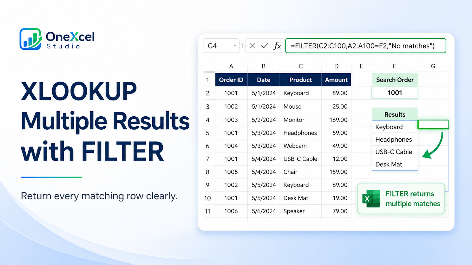
Set up the worksheet before changing it

Create a source table with Order ID, Date, Product, and Amount. Put the order to search in F2 and include at least one order with two or more lines. Keep the output area clear and decide whether the result should return one column or the entire matching record.

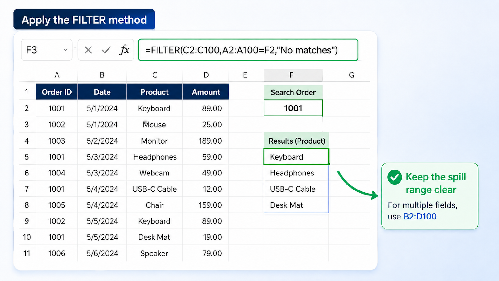
Apply the method to a real example

To return product names for the selected order, use `

`. To return several fields, change the return range to `B2:D100`. The include array must have the same number of rows as the source return range. The result spills automatically, so do not place a value directly below or beside the formula.

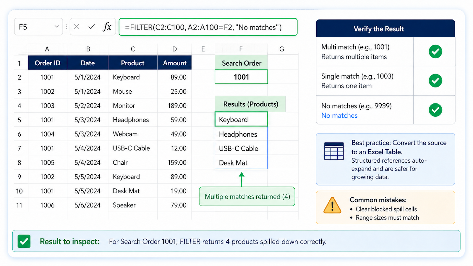
Verify the result before handoff

Test an order with multiple matches, one with a single match, and one that does not exist. Confirm the “No matches” message appears only for the last case. Add a new source row and check whether the bounded range includes it; an Excel Table with structured references is safer for a growing source. Sort the source and verify that the returned records still represent the selected order.

Common mistakes and corrections

Mistake	Correction
Using mismatched range sizes	FILTER returns an error when the include array and return array do not align.
Blocking the spill range	Clear cells below and beside the formula.
Returning only the first match	Use FILTER when the business question expects every matching row.
Using inconsistent criteria	Normalize spaces and data types in the key before filtering.

Frequently asked questions

Can FILTER return an entire row?

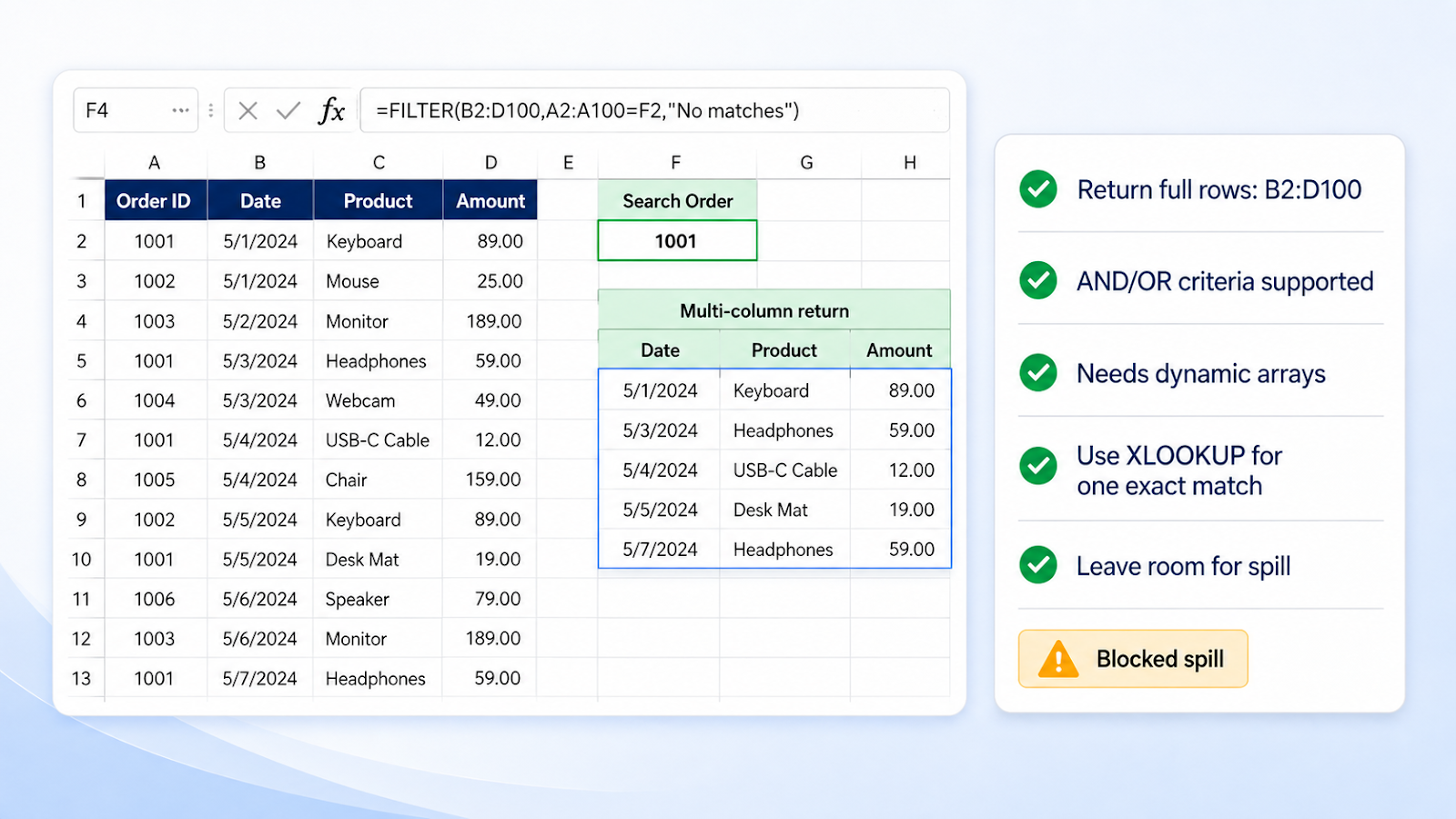
Yes. Use a multi-column return range such as B2:D100.

Can I combine multiple criteria?

Yes. Multiply Boolean tests for an AND condition, and use addition for an OR condition after testing the logic.

Does FILTER work in older Excel versions?

It requires a version that supports dynamic arrays.

When should I still use XLOOKUP?

Use XLOOKUP when the key is unique and exactly one related result is expected.

Continue with the OneXcel Tutorial Hub and free Excel resources for related workflows.

Make a multi-result lookup readable

Give the spilled result a heading and enough room to grow. If the result is used in a dashboard, show a message for no matches and consider a count beside the output. For a growing source, structured references reduce the risk that a new transaction falls outside the formula range. Review the spill after sorting and filtering the source.

Return all matching records safely

When one key can have several transactions, the output should make the multiplicity visible. Add a heading above the spill range and, when helpful, a count such as =ROWS(FILTER(B2:B100,A2:A100=F2,"")). The count helps a reader distinguish one result from a group of results.

For multiple criteria, combine Boolean tests carefully. For example, filter rows where Order ID equals F2 and Product equals G2. Test blank criteria and normalize text before comparing. If the source is an Excel Table, structured references make the formula easier to maintain as new transactions arrive.

Keep the spill area clear and test the output after sorting the source, adding a row, and searching for a missing key. These checks prove that the formula returns the intended records rather than merely producing a plausible list.

Make the result hold up in real work

Dynamic formulas can return more than one row, so decide whether the result belongs in a spill area or needs a single summary. For XLOOKUP, confirm the lookup key is unique or define which match should win. For FILTER, test zero results, multiple results, and criteria containing blanks. Use an Excel Table when new rows should be included automatically, but keep the spill destination clear. A formula that works on a five-row sample may fail when another record is added beside the output. Check the resulting range before placing labels, totals, or other formulas next to it.